MSc Computer Science Dissertation · University of Zimbabwe · 2026

Gold Prospectivity Mapping in Bindura, Zimbabwe

Can machine learning find gold when you only have four known deposits to learn from? This study compares One-Class SVM, Isolation Forest and XGBoost under identical conditions across the Bindura greenstone belt — and shows that in data-scarce terrains, the data, not the algorithm, decides the outcome.

The problem

Zimbabwe's greenstone belts are richly mineralised but thinly explored. Modern prospectivity mapping assumes dozens of labelled deposits and dense geochemical grids. Bindura offers neither. This dissertation tests what actually happens when established machine learning methods meet that reality — and which of them degrades gracefully.

4
verified gold deposits used as training labels
14
integrated predictor variables in the feature stack
51,134
pixels classified across the study area
≈46 km²
of mid-Bindura District modelled
3
algorithms compared under identical conditions

Results

Each model produced a per-pixel prospectivity surface over the same feature stack. Only one produced a map an exploration geologist could act on.
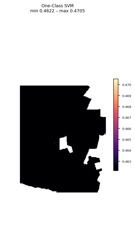
One-Class SVM prospectivity map showing near-uniform values across the study area
Failed

One-Class SVM

Assigned effectively the same probability to every pixel. No spatial discrimination — the map carries no exploration signal at all.

Range 0.4622 – 0.4705 · spread 0.008
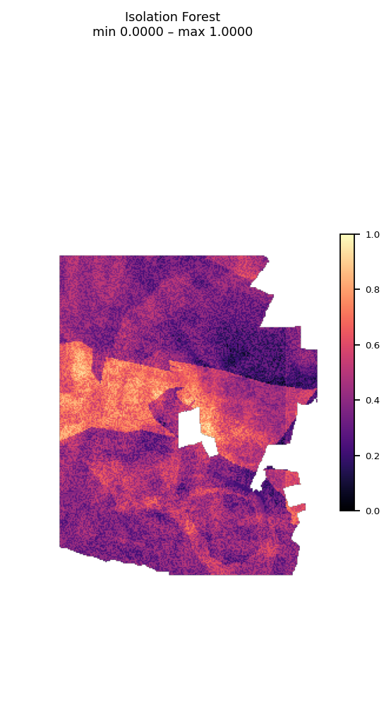
Isolation Forest prospectivity map showing clear high-value corridors
Best performer

Isolation Forest

Clear separation between prospective and non-prospective zones, resolving a coherent east–west high-prospectivity corridor. Delineated 6.9 km² of high-priority targets — 14.98% of the study area.

Range 0.000 – 1.000 · mean 0.446
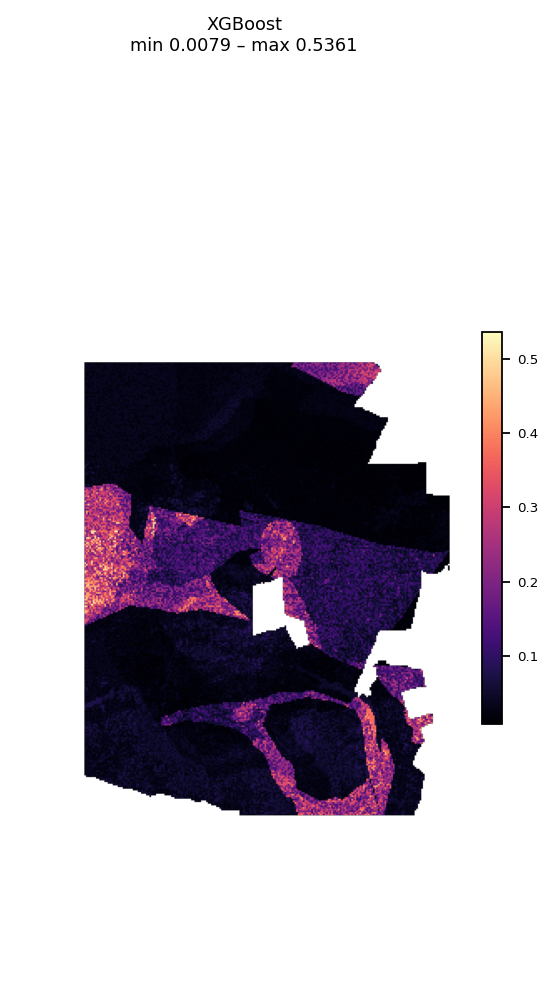
XGBoost prospectivity map showing consistently low probabilities
Over-conservative

XGBoost

Produced 3,413 distinct probability values — genuine variation — but pressed almost all of it into the low range, leaving no confident targets to follow up.

Range 0.008 – 0.536 · mean 0.071
The finding that matters. The two failures were not algorithmic. Four training deposits, sparse geochemical sampling requiring extensive interpolation, and incomplete spatial coverage explain them far better than any property of SVM or gradient boosting. With 30–50 deposits and systematic grid sampling, all three would likely perform substantially better — and probably comparably.

Method

Identical preprocessing, identical inputs, three independent Python scripts.

  1. Assemble the feature stack. Fourteen co-registered predictor bands — geology, structural controls, geochemistry, remote sensing indices and terrain — built and aligned in ArcGIS.
  2. Interpolate the geochemistry. Empirical Bayesian Kriging across sparse sample points to produce continuous element surfaces (Au, As, Sb, Cu, Zn, Fe).
  3. Define training labels. Four verified gold deposits; historical mine locations retained for reference and qualitative validation.
  4. Train and predict. Each algorithm trained and applied independently over the same stack, emitting a 0–1 prospectivity value per pixel.
  5. Compare. Outputs assessed on spatial discrimination, value distribution and high-priority target area.
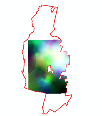
The 14-band feature stack used as model input

The integrated 14-band feature stack.

Code, data and documents

Everything reproducible is in the repository. The multi-gigabyte GIS dataset is archived separately.

Source code

Four ArcPy scripts — one per model, plus the comparison routine.

Prospectivity maps

Georeferenced GeoTIFFs (EPSG:4326, 274 × 557 px), one per model.

Sample data

Mine locations, geochemical sample points and element statistics.

Workflow guides

EBK interpolation in ArcMap and ModelBuilder setup.

Full dataset

Geodatabases, DEM and rasters — archived on Zenodo with a citable DOI.